Design Of Experiment (DOE)
- jjinghui21
- Jan 21, 2023
- 5 min read

Hello it's been a while, in this blog I will be documenting and describing how I will perform full factorial and fractional factorial data analysis to solve a case study. I will also be sharing my personal learning reflection for the practical session.
CASE STUDY
What could be simpler than making microwave popcorn? Unfortunately, as everyone who has ever made popcorn knows, it’s nearly impossible to get every kernel of corn to pop. Often a considerable number of inedible “bullets” (un-popped kernels) remain at the bottom of the bag. What causes this loss of popcorn yield? In this case study, three factors were identified:
Diameter of bowls to contain the corn, 10 cm and 15 cm
Microwaving time, 4 minutes and 6 minutes
Power setting of microwave, 75% and 100%
8 runs were performed with 100 grams of corn used in every experiments and the measured
variable is the amount of “bullets” formed in grams and data collected are shown below:
Factor A= diameter
Factor B= microwaving time
Factor C= power
Run order | Factor A | Factor B | Factor C | Bullets (grams) |
1 | + | - | - | 3.64 |
2 | - | + | - | 2.64 |
3 | - | - | + | 0.74 |
4 | + | + | - | 1.64 |
5 | + | - | + | 0.95 |
6 | + | + | + | 0.32 |
7 | - | + | + | 0.64 |
8 | - | - | - | 3.12 |
Hyperlink to excel for both full and fractional factorial data analysis:
Full Factorial Data Analysis


When the diameter of bowls to contain the corn (factor A) increases from 10cm to 15cm the average mass of the bullets decreases from 1.79g to 1.6375g.
When the microwaving time (factor B) increases from 4 minutes to 6 minutes, the average mass of the bullets decreases from 2.11g to 1.31g.
When the power setting of microwave (factor C) increases from 75% to 100%, the average mass of the bullets decreases from 2.76g to 0.6625g.
Factor C has the steepest gradient followed by B then A
Most significant factor | -> | Least significant factor |
Power (C) | Time (B) | Diameter (A) |
Interaction effect:

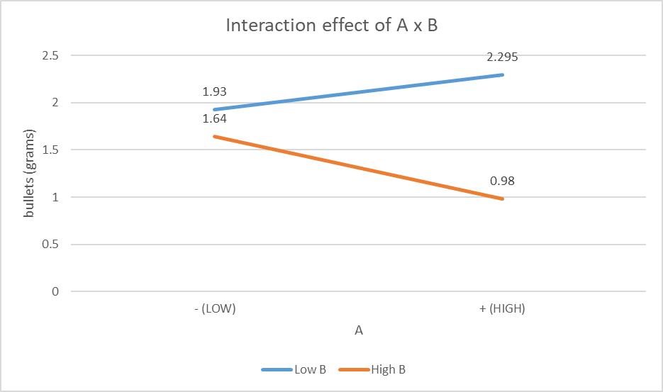
The gradient of both lines is different. The gradient of low B is positive while the gradient of high B is negative. Even though in this graph they do not intersect, there is significant interaction between factor A and B as they will eventually meet since they are not parallel.


The gradients of both lines are negative but they are slightly different as both lines are not parallel. Since both lines are almost parallel, there is small interaction between factor A and C.

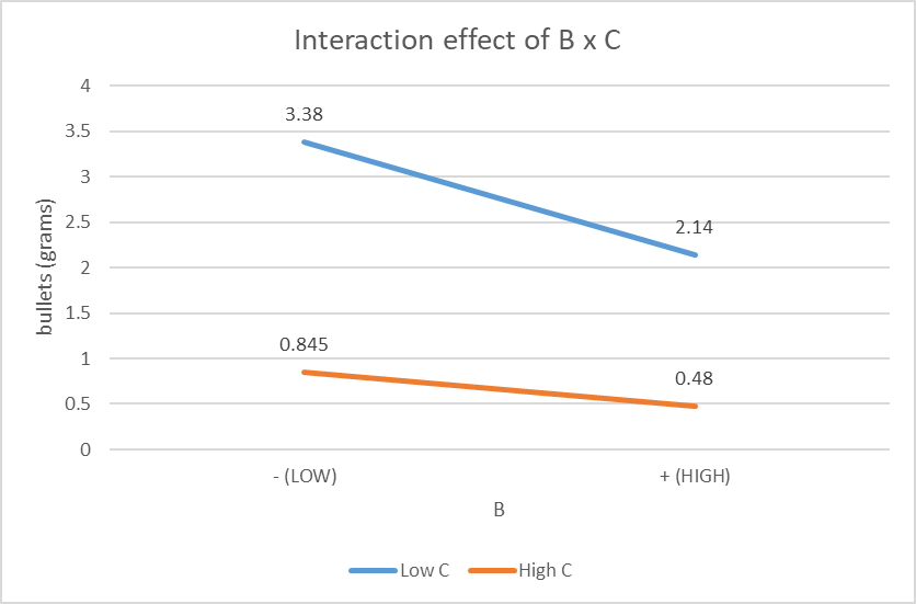
The gradients of both lines are negative, but they are different and both lines are not parallel. Compared to A x C, B x C has a larger interaction as the difference in gradient is larger. However, the interaction between factor B and C is still considered small as the lines are not intersecting but they will eventually meet since they are not parallel.
Conclusion:
Factor C, Power of the microwave is the most significant factor and has the least interaction with the other two factors.
Fractional Factorial Data Analysis
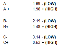
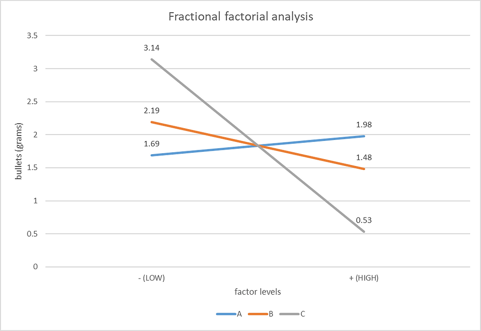
When the diameter of bowls to contain the corn (factor A) increases from 10cm to 15cm the average mass of the bullets increases from 1.69g to 1.98g.
When the microwaving time (factor B) increases from 4 minutes to 6 minutes, the average mass of the bullets decreases from 1.843g to 1.490g.
When the power setting of microwave (factor C) increases from 75% to 100%, the average mass of the bullets decreases from 2.098g to 1.235g.
Factor C has the steepest gradient followed by B then A
Most significant factor | -> | Least significant factor |
Power (C) | Time (B) | Diameter (A) |
Despite having missing information, the graphical trend for fractional factorial data analysis is the same as the full factorial data analysis.
Interaction effect:
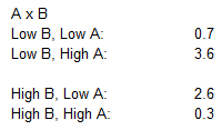
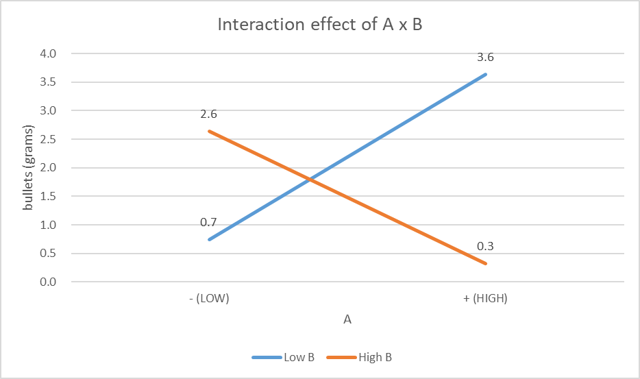
The gradient of both lines is different. The gradient of low B is positive while the gradient of high B is negative. In this graph the lines intersect, therefore there is significant interaction between factor A and B.
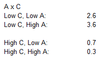
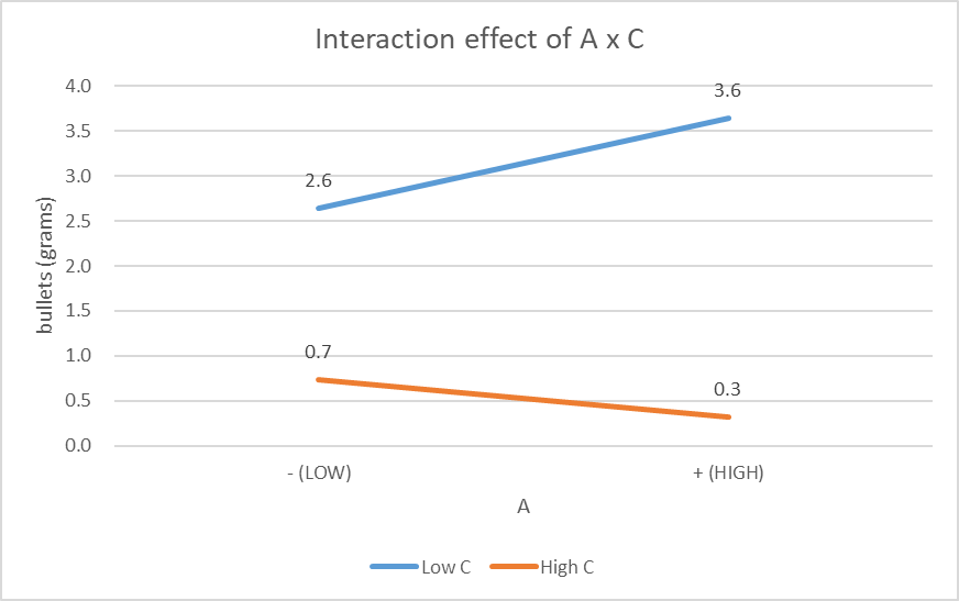
The gradient of both lines is different. The gradient of low B is positive while the gradient of high B is negative. They do not intersect, therefore compared to A x B, A x C has a smaller interaction. There is small interaction between factor A and C as they will eventually meet since they are not parallel.
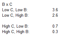
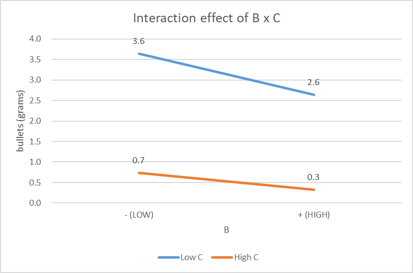
The gradients of both lines are negative, but they are different and both lines are not parallel. There is small interaction between factor A and C as they will eventually meet since they are not parallel. There is small interaction between factor B and C as they will eventually meet since they are not parallel.
Conclusion:
For this fractional factorial data, it is very similar to the full factorial data with some difference in the interaction effect graphs and it has the same trends. Factor C, Power of the microwave is still the most significant factor and has the least interaction with the other two factors.
PERSONAL LEARNING REFLECTION
During the tutorial session, I could understand how DOE works as we had applied in last year in LPS2 where we had to conduct leaching using coffee with different factors assigned to each group. I felt that as long as I followed the slide and the excel guide, I can't go wrong with my calculations and my graphs will be correct.
When it came to topic 7-2, I initially very confused on how the interaction effect works, like how can numbers (data values) tells you they interact.
However, the slides used an example where stirrer speed, temperature and diameter are the factors.
I felt that it helped me understand interaction effect better as I know that when we stir something hot, it cools it down faster. Hence, with the help of prior knowledge, I kind of understand interaction effect.

During the practical session, we conducted experiments where we used catapults to launch a ball. Each run was repeated 8 times and we had changed some factors. DOE was then applied to determine the most significant factor (spoiler: it was the stop angle). The execution of the experiment was pretty simple, the more taxing task would be the somewhat new skill of DOE to obtain data.

Next, we had a challenge where we needed to knock down our lecturers and had to compete against other groups. We all knew that going last had more advantage, however, if there wasn't any group willing to go first when would this challenge even start? Hence, our group decided to go first as we thought we can just hit one and like come back later. little did we know once we started, we could not stop...
Below is a video of our first hit which was our first trial:
We were so happy and excited here (this was before we realize we can't step away and continue calculating/planning)
We also wasted 2 trials on sure hits. Other groups saw this and did not use their trials on targets they were confident in. Our blunder became a steppingstone to their success. We were all very salty about this >:((
In the end, we tied with another group with 2 hits while the other 2 groups had 4 hits.
I believe that my group could have hit all 4 lecturers if we hadn't gone first and had the chance to observe others. Observing others would have allowed us to not make the same mistakes as them and given us more time to plan our shots.
I truly regretted attempting to be the "sacrifice" group of the class. I have learnt that sometimes it is important to be selfish and put yourself first before others. Especially in a competition.




Comments